It has been established that Rayleigh lidar systems, like ARCLITE, can provide precise middle atmosphere temperature profiles, assuming hydrostatic equilibrium and the ideal gas law, at high spatial resolution on a routine basis [e.g., Kent and Wright, 1970; Hauchecorne and Chanin, 1980; Russell and Morley, 1982]. The temperature retrieval technique we employ, described by Hauchecorne and Chanin [1980], is where the temperature at height in a layer thickness of is given by

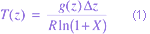
where is the gravitational acceleration at altitude is the gas constant for dry air, and is expressed as

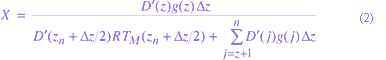
where is the modified relative density given as

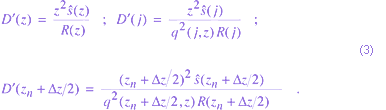
The expression for illustrates that the lidar-derived temperature profile is dependent only on the relative density profile when a model temperature, provided by MSIS-90 for example, is used at the top of the n^th layer or upper bound layer . As shown by Russell and Morley [1982], if a model pressure is used at the top of the n^th layer instead of temperature, the lidar-derived temperature profile is also dependent on the factor , where is the index for the normalization altitude used to obtain the lidar-derived density profile. Thus, a temperature value used at the upper bound of the profile instead of pressure avoids the additional uncertainty in determining the density at the lower normalization altitude. The temperature relative error, employing propagation of error techniques, that we use in our analysis is written as



where



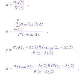
with



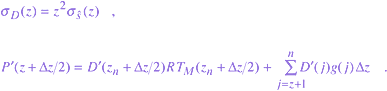
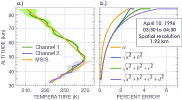
Figure a.), above, is an example of a lidar-derived temperature profile and its associated error with 60-minute integration and 0.96 km vertical resolution. The MSIS-90 temperature profile for this day is given by the dashed line. A pervasive feature in this temperature profile and many others determined from ARCLITE is the presence of gravity waves. Further study concerning leewave sources of gravity waves at the site and variations in gravity wave activity determined from the lidar data are underway. The contribution of each of the error terms , , , and in Eq.(4) is shown by Figure b.). The figure shows the cummulative error estimate in terms of percent error versus altitude with the net error needing to be scaled by the factor ,which for this case was near 0.94, to get the complete temperature error. The greatest contribution to the temperature error comes from the relative error of the signal, , with the downward-integrated signal error increasing its contribution as the integration is extended from the upper bound altitude of 95 km to lower altitudes. The error estimate associated with the upper bound parameters, and , using a model temperature error of 20 K, influences the temperature error within the first 10 km from the upper bound, as was also found by Hauchecorne and Chanin [1980]. As a result, in practice we set the altitude of the upper bound to be constrained to a signal percent error between 15 and 20%, which is typically 10 km above the altitude of interest.

Noctilucent Cloud Observations